How To Highlight Duplicates In Excel? Users must Know

Before you proceed to this article, you need to accept that your excel sheet has some errors and duplicates. Many times, when you feel data in the sheets, it may create duplicates in the file. That’s why it’s essential to find duplicates in the sheet and highlight them. In this article, you will learn how to highlight duplicates in Excel. So, it will help you filter out your data and qualify your sheet for further assessment. Let’s start with understanding the basics of duplicates, highlighting them in the sheet, and how to purify your file.

Overview:

Let’s assume you have created a list of supermarkets in the country that sells foods and vegetables. The list will also include the types and categories of foods and vegetables, their prices, quality, and lots of things. However, many times it happens that you mistakenly enter any values two times. Say, for example, price. Now, when the list is too long, it’s technically not convenient to read all data and find duplicate values to delete it. That’s why excel lets you find the duplicates and highlight them to make your datasheet accurate. It also lets you permanently delete duplicate content.

How To Highlight Duplicates In Excel?

There are two ways to highlight duplicates in Excel. The first is a single Excel column, and the second is an entire worksheet. It depends on how you select the cells. So, it’s very important to select the column carefully. Let’s understand it with a few examples.

Highlighting Current Duplicates In The Selected Range:

When you select a particular range of Excel, you can highlight duplicates in that area. The following is how to highlight duplicates in Excel for the selected range.

• Select the range of data you need to check.
• Click on the command of CONDITIONAL FORMATTING.
• Go to its drop-down menu and navigate for styles from Home Tab. 
• Find the command Highlight Cells Rules. 
• Select “Duplicate Values.”

Alternate Method:

• You can use the shortcut by Pressing Keys “Alt+H+L+H+D.” 
• It will open the dialog box for duplicate values. 
• From there, choose the required type of formatting.
• You can highlight the cell, text, or both, and the colors can be changed too! It also lets you highlight the borders of your datasheet cells that have been Duplicated.
• Further:
• Select the option “Light Red Fill With Dark Red Text.”
• Click on OK.
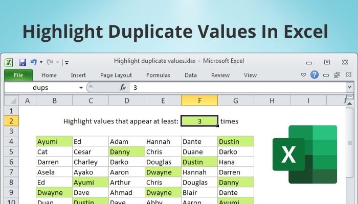
• It will highlight the duplicate values in the selected range of your datasheet, but remember that the CONDITIONAL FORMATTING feature will highlight all the data having duplicates, even with the first one.

How To Highlight Future Duplicates In Your Datasheet For Selected Range?

Let us assume your datasheet may have duplicate values in the future too! That’s why it’s essential to know to avoid it. But you can also pre-plan to highlight that part of your datasheet. Here, the CONDITIONAL FORMATTING feature will help you. The following is the process.

• Select the column number you want to monitor. It makes it easier to highlight the new duplicates in the future.
• Go to Home Tab and navigate for conditional formatting.
• Click on the drop-down menu and select styles. 
• Choose Duplicate Values and Highlight Cells Rules.
• Prefer the duplicate values color and select “Green Fill With Dark Green Text.” You can choose your preferred color.
• Click on OK.
• It will show you the number of duplicate values in the file that is more than one.
• Enter the number of your data in the row with the selected column, and it will automatically highlight future duplicates.

Things To Consider:

You can also select your entire file in the first step and proceed with steps two and further. It will let you obtain duplicates in the entire file.

Do you know that selecting a specific section and an entire worksheet differ? If you select a particular range, it will only highlight future duplicates in that area, but the entire select file will give a highlight to any duplicate data. 

How To Remove Duplicates From Selected Range?

Now, you have understood how to highlight duplicates in Excel, but that’s not a done task because you also want to delete the duplicates from the selected area to keep your file clean. Removing duplicates from a selected range of datasheets is done as under.

• Select your worksheet’s range.
• Click on “Remove Duplicates.” It is available in Data Tools. Find it under the section Data Tab. 
• The shortcut key to remove duplicates is “Alt+A+M.”
• You will see a dialog box asking the confirmation about deleting the duplicates from the selected range.
• Also, remember to check the checkbox “My Data Has Headers.” 
• Click on OK.
• It will remove the duplicate values from the selected range of the column. 
• It will show you the message stating the number of duplicates deleted from your selected range of datasheets.
• You will notice the unique data only then.

Beware Of Governing Duplicates In Excel:

While finding and deleting duplicates in Excel, you must take care of the following points.

• Don’t forget to ensure that you have selected the appropriate range of datasheets to highlight duplicates.
• Remember that you must select Custom Format from the Duplicate Values section.
• Also, remember to choose the Current Column Header while removing your duplicates in Excel.

What Is Highlight In Excel?

Excel datasheet has duplicate values more than once. We use the highlight feature to understand the data and make it pure. Once you know how to highlight duplicates in Excel and do it, you can find all duplicates and remove them from your worksheet.

Can You Highlight Duplicates In Multiple Columns?

Yes! You can select all columns without the doubt of having duplicate values. Here are the steps to do it.

• Choose the range of datasheets with several columns and rows.
• Go to CONDITIONAL FORMATTING and select Duplicates.
• Navigate to FORMAT and choose the color.
• Click on OK. 
• You will see a new formatting rule. Click on OK. That’s the easiest way to find duplicates from multiple columns and rows and highlight them in your current datasheet.
• Once the rule is applied to the selected range, you will see a dialog box of CONDITIONAL FORMATTING RULES MANAGER.
• Click on OK for this manager.
• Hence, your task is done. You can successfully select and highlight the Duplicates that occurred in multiple columns and rows. 

How To Highlight Duplicates In Excel With Excel Formula?

Before you do it, you must know that excel has the facility to let you use the excel Formula that easily highlights duplicates in Excel. If you don’t want to go through the manual process, you can use the COUNTIF Formula by following the steps. 

• Choose the range of datasheets you need to check for Duplicates In Excel.
• Go to CONDITIONAL FORMATTING. Find it under the Home Tab.
• Choose New Rule.
• It opens the window of the New Formatting Rule.
• Navigate for the USE A FORMULA TO DETERMINE CELLS TO FORMAT option.
• Go to EDIT THE RULE DESCRIPTION. 
• Enter the formula =COUNTIF (Range,to_cell)>1.

Let’s Explain The Terms From This Formula:

• The range is the selected range of your datasheet. 
• Top_Cell is the first, leftmost cell of your currently selected range.
• When the range is like A1:C8, you must write the formula =COUNTIF ($A$1$C$5, A1)>1.
• Now, go to the FORMAT.
• Select your preferred color. Find it under Fill Tab. It is used for highlighting Duplicates In Excel.
• Click on OK, and again click OK for the NEW FORMATTING RULE Window.
• This way, you can highlight duplicates in Excel for the selected range of datasheets with the help of Excel Formula.

What Is Best? Highlighting Duplicates In Excel Manually Or Using An Excel Formula?

We discussed two of the main points about Excel datasheets. The first is how to highlight duplicates in Excel Manually, and the second is how to highlight your duplicates in Excel datasheet with the help of Excel Formula. Both methods have their unique advantages. No matter what you use, keep in mind the following points.

• Both methods are accurate in highlighting and deleting Duplicates In Excel. Of course, you can trust both features.
• Don’t think that Highlight Duplicates In Excel With Excel Formula will not give correct results because it includes the selected range of datasheets, and that’s why the results are perfect.
• You can use any of these two methods to highlight duplicates in Excel based on your skills and expertise. Some users prefer formulas, and some go with the manual process.

Wrapping Up:

Did you understand two ways of Highlighting Duplicates In Excel? If you don’t know how to highlight duplicates in Excel, this article has helped you a lot. Always consider safety things about deleting or removing duplicates in Excel because once you lose data, it won’t 

come back if saved. That’s why select only the doubtful range of datasheets from your Excel file to avoid mistakes. Did you find this answer helpful? If you have successfully highlighted and removed Duplicates In Excel, let us know in the comment to encourage readers to know these two ways and use them more efficiently.

Puspa

I m a passionate blogger. I have completed my MBA in IT and marketing also worked as an SEO Executive for 3 years. Now I v around 2 years of experience in writing content with multi-directional topics. I used to spend a lot of time surfing to getting exposed to the multi-topics & day to day arena of knowledge. My words have touched millions of people. Basically, I put love into words and help you connect to matters thoroughly and simply.